Arc-length Parameterisation Made Easy

Arc-length parameterisation is a topic that is often introduced right at the beginning of any course on differential geometry or multivariate calculus, the reason behind this is that it’s a relatively simple concept and it’s core to defining curvature, Frenet frames and some other central important concepts.

In the context of this being an introductory and foundational part of any course on differential geometry you might be surprised to find that the standard notation used when discussing arc-length parameterisation is highly confusing and inconsistent. I can only assume that this notation was picked some time ago, as it has appeared in every course or textbook I’ve seen on the topic in the exact same way. At the end of the this post I’ve outlined the issues I have with the standard notation in more detail, for now however, I’ve gone through some of the very introductory definitions with a consistent notation and a (in my opinion) more understandable approach. Nothing here is new or particularly interesting, but if you also find the notation for arc-length parameterisation frustrating, I hope this helps.

Curves and parameterisations

Definition: A curve is the image of a function from some interval $I = [a, b] \subset \mathbb{R}$ to $\mathbb{R}^n$.

For example, if $I = (0, 2\pi)$ and $X(t) = (\sin(t), \cos(t))$, the image of this function is the unit circle, so we would consider the unit circle a curve in this context. In this example $X$ is a parameterisation of the curve.

Velocity and acceleration vector image

It’s important to note that the same curve can have multiple parameterisations. For example, the image of the function $Y(t) = (\sin(2t), \cos(2t))$ on the interval $(0, \pi)$ is also the unit circle, but $X$ and $Y$ are clearly different functions.

We often write curve parameterisations in terms of their component functions: \[X(t) = (x_1(t), x_2(t), \dots, x_n(t))\]

We can define addition, scalar multiplication and dot product on curve functions which operate as you would imagine:

$X(t) + Y(t) = (x_1(t) + y_1(t), x_2(t) + y_2(t), \dots, x_n(t) + y_n(t))$.
$X(t) = (cx_1(t), cx_2(t), \dots, cx_n(t))$.
$X(t) \cdot Y(t) = x_1(t)y_1(t) + x_2(t)y_2(t) + \dots + x_n(t)y_n(t)$.

A useful identity to keep in mind throughout is that the standard Euclidean norm of a vector can be written as the square root of the dot product with itself

\[\|X\| = \|(x_1,x_2,\dots,x_n)\|= \sqrt{x_1^2+x_2^2+\dots+x_n^2} = \sqrt{X \cdot X}\]

Therefore $\|X\|^2 = X \cdot X$.

Curve differentiation

Let $X(t)\colon I \to \mathbb{R}^n$ be a curve parameterisation. We can write $X(t)$ in terms of its coordinates:

\[ X(t) = (x_1(t), x_2(t), \dots , x_n(t)) \]

We say that $X(t)$ is differentiable if $x_i(t)$ is differentiable for every $i$ and define the derivative of $X$ as:

\[ X’(t) = (x_1’(t), x_2’(t), \dots , x_n’(t)) \]

Here’s a few identities for curve derivatives that will be useful.

Product rule for scalar functions: If $f\colon I \to \mathbb{R}$ is defined on the same interval $I$ as a curve parameterisation $X(t)\colon I \to \mathbb{R}^n$ and $f$ and $X$ are both differentiable, then we find that \[ \frac{d}{dt} f(t)X(t) = f’(t)X(t) + f(t)X’(t)\]
Product rule for dot products: If $X\colon I \to \mathbb{R}^n$ and $Y\colon I \to \mathbb{R}^n$ are two differentiable curve parameterisations defined over the same interval, then we find that: \[\frac{d}{dt} X(t)\cdot Y(t) = X’(t) \cdot Y(t) + X(t) \cdot Y’(t)\]
Chain rule for curves: If $f \colon J \to I$ is a differentiable function from an interval $J$ to another interval $I$, and $X\colon I \to \mathbb{R}^n$ is a differentiable curve parameterisation defined on $I$, then $X(f(t))\colon J \to \mathbb{R}^n$ is another curve parameterisation defined over $J$ where: \[\frac{d}{dt} X(f(t)) = X’(f(t))f’(t)\]

Velocity and speed

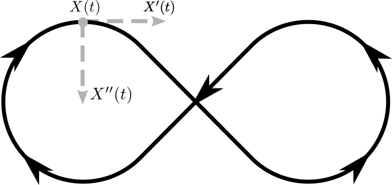
Let $X(t) \colon I \to \mathbb{R}^n$ be some differentiable curve parameterisation. Then we define the velocity vector of $X(t)$ to be $X'(t)$, and we define the speed of $X(t)$ to be $v_X(t) = \|X'(t)\|$.

If the second derivative of $X$ exists, we can define the acceleration vector of $X(t)$ to be $X''(t)$, and the acceleration to be $a_X(t) = \|X''(t)\|$.

Velocity and acceleration vector image

Example

Let $X(t) = (\sin(t), \cos(t))$ where $t \in [0, 2\pi]$ be a parameterisation of the unit circle. We can calculate the velocity vector $X'(t)$ to be: \[X’(t) = (\cos(t), -\sin(t))\] To get the speed of $X(t)$ we can then calculate the norm of this to be: \[v_X(t) = \|X’(t)\| = \sqrt{\cos^2(t) + \sin^2(t)} = \sqrt{1} = 1\]

The acceleration vector comes out to be: \[X''(t) = (-\sin(t), -\cos(t)) = -X(t)\] The norm of this function is also $1$, so the acceleration comes out to be $a_X(t) = 1$.

Curve Length

We define the length of a curve to be the integral of its velocity vector¹, much as how distance travelled is the integral of velocity in Newtonian physics.

If $X(t)$ is the parameterisation of a curve defined over $I=[a,b]$ then we define the length as: \[L(X) = \int_a^b v_X(t) dx\]

It’s a simple exercise to compute this for the unit circle parameterisation we’ve been using and you will find that that the unit circle has length $2\pi$, just as we’ve always suspected.

\[L(X) = \int_0^{2\pi} v_X(t) = \int_0^{2\pi} 1 = 2\pi\]

Re-parameterisation

We mentioned briefly at the beginning that a curve can have multiple parameterisations, lets look at some results that come from using a scalar function to get a new parameterisation.

If $f\colon J\to I$ is a surjective function from $J$ to $I$, where both $J$ and $I$ are intervals, we can combine this with a curve parameterisation $X\colon I \to \mathbb{R}^n$ to form a new curve parameterisation $Y(t) = X(f(t))$. In this case $Y$ goes from $J$ to $\mathbb{R}^n$. Importantly, the image of $Y$ is the same as the image of $X$ as $f$ was surjective, hence both $X$ and $Y$ are parameterisations of the same curve.

Notice that if $X$ and $f$ are differentiable, then so is $$Y$, and we get that \[Y’(t) = X’(f(t))f’(t)\] by the chain rule.

Most importantly, we get the result that \[v_Y(t) = \|Y’(t)\| = \|X’(f(t))f’(t)\| = \|X’(f(t))\|\|f’(t)\|\]

This is all just to show that if we have a curve parameterisation $X$, we can use a composition with a function $f$ to get a parameterisation of the same curve but with a different velocity. Now we can get to the meat of the issue: arc-length parameterisation.

Arc-length parameterisation

If we can come up with a way to take any curve parameterisation $X$ and construct an equivalent curve parameterisation $Y$ such that $v_Y(t) = 1$ for all $t$, we will find that this parameterisation gives us a lot of useful properties. This process is called arc length parameterisation. In some ways the arc length parameterisation for a curve is the parameterisation for that curve.

Let $X(t)\colon I \to \mathbb{R}^n$ be our parameterisation where $I=[a,b]$², we assume that it’s differentiable and also that $v_X(t) > 0$ for all $t \in I$.

Now we can define a function $s\colon I \mathbb{R}^n$, this function calculates how long the curve is up to a point $t$. It’s simply our length function, but not the whole way from $a$ to $b$, just $a$ to $t$.

\[s(t) = \int_a^t v_X(t)\]

It’s simple to verify that $s(a) = 0$ and $s(b) = L(X)$, so the domain of $s$ is $I$, and the image is $[0, L(X)]$.

By the fundamental theorem of calculus, we can see that $\frac{d}{dt}s(t) = v_X(t)$. From our earlier assumption, $v_X(t) > 0 \; \forall\ t \in I$. This tells us that $s$ is a strictly increasing function, which immediately implies that it is injective, and hence bijective between $I$ and $[0, L(X)]$. Therefore $s$ has a differentiable inverse $s^{-1}$:

\[s^{-1}\colon [0, L(x)] \to I\].

It turns out this is the exact function we need to convert our parameterisation $X$ into an arc-length parameterisation. We define this parameterisation as: \[Y(t) = X(s^{-1}(t))\] This parameterisation is defined over $[0, L(x)]$. Let’s verify that $v_Y(t) = 1$ for all $t$ as we desire.

Verification

As we saw earlier, the chain rule tells us that

\[v_Y(t) = \|Y’(t)\| = \|X’(s^{-1}(t))\|\|s^{-1’}(t)\|\]

where $s^{-1'}(t)$ is the derivative of $s^{-1}$ w.r.t. $t$.

By the inverse derivative rule we get that $s^{-1'}(t) = \frac{1}{s'(s^{-1}(t))}$³.

Remembering that $s'(t) = v_X(t) = \|X'(t)\|$ we can simplify this to:

\[v_Y(t) = \|X’(s^{-1}(t))\|\|s^{-1’}(t)\| = v_X(s^{-1}(t))\left\Vert\frac{1}{v_X(s^{-1}(t))}\right\Vert\]

We know that $v_X(t) > 0$, so we can eliminate the norms and get:

\[v_Y(t) = v_X(s^{-1}(t))\left\Vert\frac{1}{v_X(s^{-1}(t))}\right\Vert = 1\]

Therefore $v_Y(t) = 1$ for all $t$ as we required, and this parameterisation is arc length parameterised.

Some Useful Properties

Now that we have our parameterisation $Y(t)$ with $v_Y(t) = 1$, what can we do with this information?

Osculating Plane

The first thing to note is that since $v_Y(t) = 1$, then $v_Y(t)^2 = 1$. This allows us to calculate:

\[v_Y(t)^2 = \|Y’(t)\|^2 = Y’(t) \cdot Y’(t) = 1\]

Taking the derivative of both sides of this expression (assuming second derivates exist) with the product rule for dot products gives:

\[Y’(t) \cdot Y’(t) = 1 \implies Y’(t) \cdot Y''(t) = 0\]

Therefore the velocity vector and the acceleration vector are perpendicular at every point on the curve. This allows us to define a plane at every point, this is known as the osculating plane. It turns out this plane isn’t dependent on the specific parameterisation $Y$. Returning to our definition for $Y$: $Y(t) = X(s^{-1}(t))$, we can compose each side with $s(t)$ to find

\[Y(s(t)) = X(s^{-1}(s(t))) \implies X(t) = Y(s(t))\]

Taking the first and second derivates of $X$ (assuming they exist as usual) we get

\[X’(t) = Y’(s(t))s’(t)\] \[X''(t) = Y''(s(t))s’(t) + Y’(s(t))s''(t)\]

Remembering that $s$ is a scalar function, we can see that both the velocity and acceleration vectors of $X$ are linear combinations of the velocity and acceleration vectors of $Y$. This means that all these vectors lie in the osculating plane as defined by $Y$. The arc-length parameterisation just gives us a standard orthogonal basis for this plane.

Curvature

The arc-length parameterisation of a circle of radius $r$ is given by:

\[Y(t) = \left(r\sin\left(\frac{t}{r}\right), r\cos\left(\frac{t}{r}\right)\right) \]

Feel free to check that $\|Y'(t)\|=1$.

Calculating the acceleration of this curve we find that

\[Y''(t) = -\left(\frac{1}{r}\sin\left(\frac{1}{r}\right), \frac{1}{r}\cos\left(\frac{1}{r}\right)\right)\] \[\implies a_Y(t) = \left\Vert\left(\frac{1}{r}\sin\left(\frac{1}{r}\right), \frac{1}{r}\cos\left(\frac{1}{r}\right)\right)\right\Vert = \frac{1}{r}\]

The acceleration of the parameterisation is $\frac{1}{r}$, which implies $r = \frac{1}{a_Y(t)}$. This also tells us that the higher the acceleration, the more smaller the radius is, and hence the more curved it is. For this reason we defined the curvature $\kappa(s) = a_Y(s)$.

The neat trick we do now is we take these facts from the circle of radius $r$ and extend them to any arc-length parameterisation of a curve. Specifically we define

Curvature: The curvature $\kappa(t)$ at a point $Y(t)$ is defined to be the length of the acceleration vector at that point: \[\kappa(t) = \|Y’‘(t)\| = a_Y(t)\]
Radius of curvature: The radius of curvature $R(t)$ at a point $Y(t)$ is defined to be the inverse of the curvature: \[R(t) = \frac{1}{\kappa(t)}\]

What is different in the standard notation?

<Rant>

There are three primary problems I have with the way that arc-length parameterisation is portrayed in the standard notation in courses and textbooks.

The use of implicit inverse functions. In the derivation of the arc-length parameterisation we define the partial length function $s(t)$. In the standard notation, rather than writing $s^{-1}(t)$, or defining a new function e.g. $f$ to be the inverse, the notation $t(s)$ is used. This might just be my CS / Programming Language background but this is absolutely wild to me. May the god’s have mercy on whoever came up with that notation.
As an extension of the above point, often the “$(t)$” part of $s(t)$ is dropped entirely, and just $s$ is used (e.g. $Y(s)$, $\kappa(s)$ etc.). This would be fine if you assume incorrectly that the intent here is that $s$ is just a variable standing for any real number in the domain, but you’d be surprised then when $Y(s)$ is differentiated with respect to t, referring back to the $t$ variable of the original parameterisation.
This is pretty standard gripe for people to have with notation, but there is heavy abuse of Leibniz notation in a lot of introductions to this concept. Treating Leibniz notation like fractions, cancelling d’s, taking inverses etc. Sometimes this is used to mask a long detailed “formal” derivation, but in this case I don’t find that to be true at all, the proofs taking a less laissez-faire approach are barely longer or harder to understand at all.

</Rant>

Technically the length as defined here depends on the specific parameterisation, which is contrary to what we would ideally want for a length definition, but in practice you can define restrictions on the parameterisation that result in all valid parameterisations giving the same length. You need at least parameterisations that are injective, and have $v(t) > 0$ for all $t$. ↩
Or $(a, b)$ or $(a, b]$ or $[a, b)$, it doesn’t matter. ↩
This comes straight out of the chain rule. Differentiate both sides of $s(s^{-1}(x)) = x$. ↩